How I Serve My LLM So That My LLM Serves Me
I have recently fine-tuned a large language model (LLM) and now I need to serve it efficiently so that I can evaluate it on the Tau benchmark.
I. Preamble
The current way I’ve been evaluating the model is to load on a server with a GPU and run single turn queries against it. This is functional and fast, but Tau is a multi-turn benchmark, so I need to be able to serve the model in a way that allows for multi-turn conversations. This is different from single-turn because the model will be acting as a user and the assistant, so the conversation tracjectories are not known in advance. This means I can’t just batch up a set of known prompts and run them through the model. I need to be able to handle concurrent requests, maintain context for the conversation and process requests quickly and cheaply.
For context, I’ve already done a few things to make the model efficient:
-
Finetuned the model using LoRA. Low order Rank Adaptation (LoRA) weight updates reduces the power/rank of a matrix to by representing the weight update with two smaller matrices , where and , which reduces the number of trainable parameters from 1M to say 16,000 where . The reason this works is because these two matrix are effectively operating in an -dimensional sub-space. compresses the matrix into the subspace, then projects the changes in that subspace back up to the original space. This means that the weight update only has an effective rank of and won’t affect the higher dimensional space in the higher dimensions because the changes only affects ~1% of the dimensions.
-
Quantize the base model to 4bit (see here) which compresses the network weights by mapping high-precision numbers (say FP16) to a smaller set of discrete values (INT4). INT4 uses less memory because each number only needs 4 bits of storage compared to FP16’s 16 bits, so you can pack 4 INT4 values in the same space as one FP16 value. Imagine you have an FP16 weight like 0.8347, and you want to fit it into INT4 which can only represent 16 values (-8 to 7). To do this, you find the range of all weights in a group (say -1.2 to 1.5), calculate a scale factor (range/15 ≈ 0.18), then divide each weight by this scale and round to the nearest integer.
-
Use vLLM for offline inference, providing a high-throughput, memory-efficient inference engine with continuous batching to maximize GPU utilization. It’s essentially a drop-in replacement for standard inference with optimized CUDA kernels that can increase throughput by 2-24x and reduce computational overhead compared to naive implementations.
II. Profiling
The objective is to serve the model efficiently, so anything optimising kernels or changing layer implementations is out of scope, in this post I’m focusing on optimizing the serving setup. The first thing I want to do is profile my serving setup to confirm that the bottleneck is indeed the model inference and not something else in the stack. My current serving setup is a vLLM inference server hosted on Modal, which is a serverless platform for hosting ML models. I used the cProfile module in python to profile a single example of the tau benchmark:
uv run py-spy record -o profile.svg --format speedscope -- uv run -m tau2.cli run ...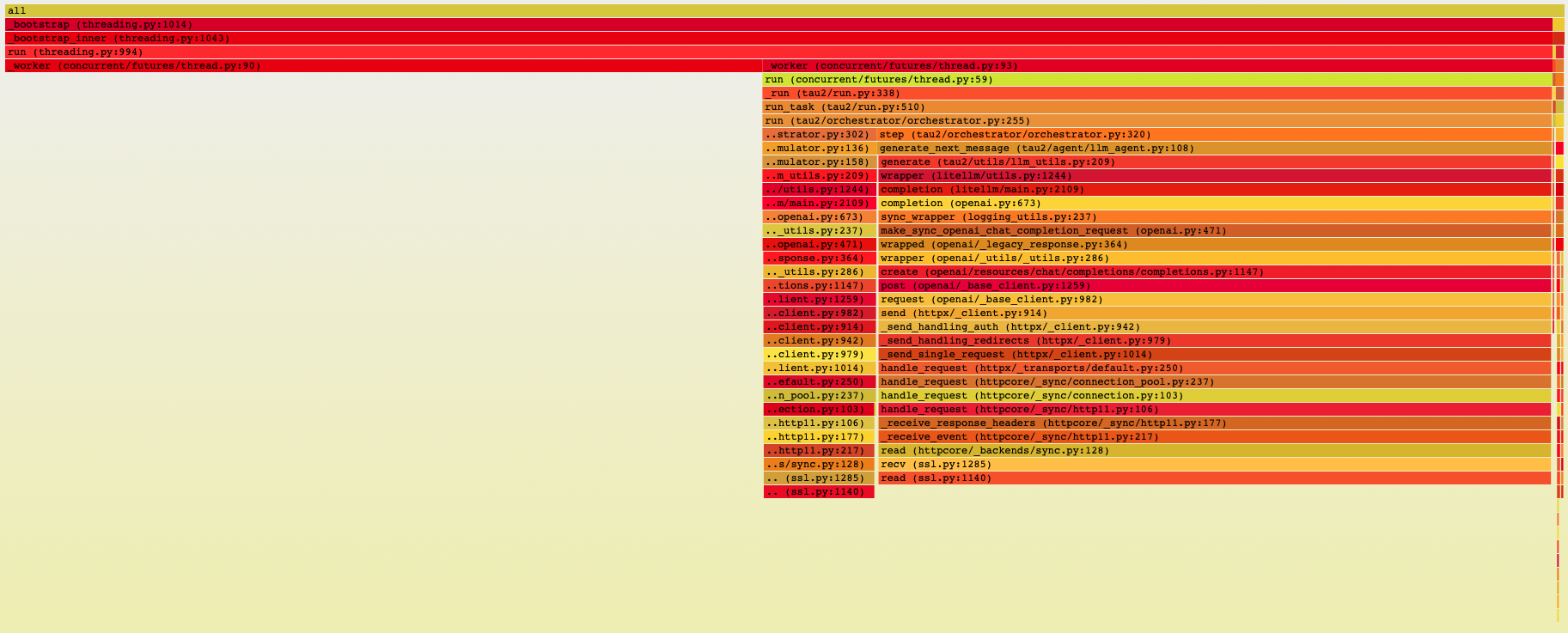
Figure 1: Profiling the tau-benchmark.
Essentially, there’s two parallel threads and most of the time is spent reading from the server, so the bottleneck is definitely the LLM.
III. Performance
Now that I knew the model inference was the bottleneck, I started tuning vLLM’s serving configuration. The first thing I did was enable KV-cache, which stores the key and value tensors from previous tokens so you don’t have to recompute them for every new token. I also enabled chunked prefill, which lets vLLM break up the initial prompt processing into smaller chunks that can be interleaved with decoding from other requests. This is particularly useful for long prompts because instead of blocking all other requests while processing a massive initial sequence, you can process a chunk, generate a token for another request, process another chunk, and so on.
The interesting question becomes: what’s the right balance between batch size and number of GPUs?
See, for real-time user-facing applications, you care deeply about latency. Every millisecond matters because there’s a human waiting for a response. But for my use case - evaluating the model on the Tau benchmark - I only care about throughput. I’m not serving real users; I’m running a massive batch job where the goal is to process as many tokens as possible as cheaply as possible within some reasonable time frame (defined by my patience which in this case is very little). This changes the optimization problem. Instead of optimizing for the fastest single-request response time, I want to maximize tokens per second per dollar.
So I ran experiments across different configurations to understand the cost vs. throughput tradeoffs:
   Cost breakdown:
   A100x8: $1.24 (4.4 minutes)
   A100x4: $0.89 (6.4 minutes)
   A100x2: $0.25 (3.6 minutes)
   H100x4: $0.90 (3.4 minutes)
   H100x2: $0.44 (3.3 minutes)
   H100x1: $0.21 (3.2 minutes)

======================================
💰 COST vs PERFORMANCE COMPARISON
======================================

    Config         Throughput (tok/s)    TPOT (ms)    Cost/1M tok
------------------------------------------------------------------
A100 C=2 B=128     2202.3 (capacity)   5.6 (latency)    $ 0.53
A100 C=4 B=64      1061.9 (capacity)   3.4 (latency)    $ 2.20
A100 C=8 B=32      1039.2 (capacity)   0.7 (latency)    $ 4.49
H100 B=256         3287.4 (capacity)   22.5 (latency)   $ 0.33
H100 C=2 B=128     2518.3 (capacity)   10.4 (latency)   $ 0.87
H100 C=4 B=64      2399.0 (capacity)   1.9 (latency)    $ 1.83
The pattern was clear: using more GPUs gave you lower latency (that TPOT column), but worse cost efficiency. The H100 B(atch)=256 configuration had the best throughput-to-cost ratio at $0.33 per million tokens, even though it had the highest per-token latency at 22.5ms. The A100x8 configuration, by contrast, cost $4.49 per million tokens - more than 10x more expensive - for better latency.. but this case I don’t care about latency so the choice was obvious: fewer GPUs, higher batch size.
But then I started getting timeout errors.
Requests would just die mid-generation, and at first I couldn’t figure out why. Then it hit me: I was running out of KV-cache memory. When you increase the batch size, each concurrent sequence needs its own KV-cache, and at some point you run out of GPU memory and the cache starts getting evicted. Once the cache for a sequence gets overwritten, that sequence takes ages and the request times out.
I needed to figure out the actual maximum batch size I could support given my memory constraints. Here’s how I calculated it:
Total Memory = Model Parameters + KV Cache + Activations + Overhead
- Model Parameters Memory
Model Memory = num_parameters x bytes_per_parameter
Bytes per parameter by precision:
- FP32: 4 bytes
- FP16/BF16: 2 bytes
- FP8: 1 byte
- INT8: 1 byte
- INT4: 0.5 bytes
Example for Qwen2.5-7B: FP16: 7B × 2 bytes = 14 GB
- KV Cache Memory (The big one for serving)
KV Cache = 2 × batch_size × num_layers × num_kv_heads × head_dim × max_seq_len × bytes_per_element
Breaking it down:
- 2x = Key + Value
- batch_size = concurrent sequences being processed
- num_layers = transformer layers
- num_kv_heads = KV heads (may be less than query heads with GQA/MQA)
- head_dim = dimension per head
- max_seq_len = maximum sequence length
- bytes_per_element = precision (2 for FP16, 1 for FP8)
Simplified formula: KV Cache ≈ 2 x batch_size x num_layers x hidden_size x max_seq_len x bytes_per_element (where hidden_size = num_kv_heads x head_dim)
Example for Qwen2.5-7B:
- Layers: 28
- Hidden size: 3584
- KV heads: 4 (uses GQA)
- Head dim: 128
- Precision: FP16 (2 bytes)
Per token per sequence: = 2 x 28 x 4 x 128 x 2 bytes = 57,344 bytes ~ 0.056 MB per token
For 4K context (4096 tokens) = 0.056 MB x 4096 = 229 MB per sequence. For batch_size=32: 229 MB × 32 = 7.3 GB.
- Activation Memory (usually small for inference)
Activation Memory ~ batch_size x seq_len x hidden_size x bytes_per_element x num_layers
For inference this is typically ~1-2 GB depending on batch size.
- Overhead
- CUDA context: ~1-2 GB
- Framework overhead: ~1-2 GB
- Total overhead: ~2-4 GB
Now let’s do the actual calculation for my setup. I’m using a single H100 with 80GB of memory, running Qwen2.5-7B at FP16 precision.1
Model Parameters:
- 7B parameters × 2 bytes (FP16) = 14 GB
KV Cache per sequence:
- Per token: 2 × 28 layers × 4 heads × 128 dim × 2 bytes = 57,344 bytes ≈ 0.056 MB
- For max sequence length of 8192 tokens: 0.056 MB × 8192 = 458 MB per sequence
Activations:
- ~1.5 GB (relatively constant for inference)
Overhead:
- ~3 GB (CUDA + framework)
Total memory budget:
- H100 total: 80 GB
- Used by model: 14 GB
- Used by activations: 1.5 GB
- Used by overhead: 3 GB
- Available for KV cache: 80 - 14 - 1.5 - 3 = 61.5 GB
Maximum batch size:
- 61.5 GB ÷ 0.458 GB per sequence ≈ 134 sequences
So theoretically I could support ~134 concurrent sequences, but in practice I set the max batch size to 128 for a nice batch size number and some safety margin. With this configuration (H100, batch size 128, chunked prefill enabled), I can now run a full Tau benchmark evaluation in under ten minutes for $0.33 per million tokens. The timeout errors are gone, throughput is maximized, and I’m not paying for GPU capacity I don’t need. Bosh.
Footnotes
-
I realized here that I was only quantizing the model during training to save memory, but I wasn’t actually serving the quantized model. This meant my inference was running at FP16 (2 bytes per parameter) instead of INT4 (0.5 bytes per parameter). This was costing me 4x more memory than necessary, but I decided to stick with FP16 for now since I had enough memory headroom and didn’t want to deal with potential quality degradation from quantization during evaluation. ↩